Overview
Concatenator is a tool for synthesizing interpretations of a sound, through the analysis and synthesis of audio grains from a corpus database. The program works by analysing overlapping segments of audio (known as grains) from both the target sound and the source database, then searching for the closest matching grain in the source database to the target sound. Finally, the output is generated by overlap-adding the best matches.
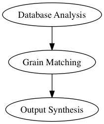
To create the final output, there are three main operations to perform:
Analysis
First, the descriptor analyses are generated for each audio file in both the source and target database. Full details on the types of descriptor available and their function can be found in the Audio Descriptor Definitions section of this documentation. Analyses are then stored to a HDF5 file, ready for matching.
![digraph b {
subgraph cluster0 {
style=filled;
color=lightgrey;
node [shape=record,width=.1,height=.1];
node0 [label = "<f0> | <f1> | <f2> | <f3> | <f4> | <f5> | <f6> ",width=2.5]
label = "Audio\nFiles";
labeljust="l";
}
subgraph cluster2 {
style=filled;
color=lightgrey;
node [shape=record,width=.1,height=.1];
node2 [label = "RMS | F0 | Centroid | Kurtosis | etc..."]
label = "Analyses";
labeljust="l";
}
database[shape=rectangle, label="Audio Directory"];
HDF[shape=rectangle, label="HDF5 File"];
database -> node0;
node0 -> node2;
node2 -> HDF
}](images/graphviz-6b757eb3efdae327054aa33b47551890084e9389.png)
Matching
Both the source and target HDF5 files are loaded to compare the values of their analyses. Each audio file’s analyses are split into equally sized overlapping grains and averaged in the appropriate way to be compared to grains from the other database. The matching algorithm then calculates the grains that have the smallest overall difference, based on user defined weightings for each of the analysis types. This weighting of analyses allows for certain analyses to gain precedence over others based on user preference. The best match indexes are then saved to the output database ready for synthesis.
There are currently two implementations for the matching algorithm:
- Brute Force
- K-d Tree Search
Both will return similar results, however the K-d tree search algorithm is far more efficient when analysing large datasets so is the preferred method.
![digraph b {
subgraph cluster0 {
style=filled;
color=lightgrey;
node [shape=record,width=.1,height=.1];
node0 [label = "<f0> | <f1> | <f2>Source | <f3>Audio | <f4>Analysis | <f5> | <f6> ",width=2.5]
labeljust="l";
}
subgraph cluster1 {
style=filled;
color=lightgrey;
node [shape=record,width=.1,height=.1];
node1 [label = "<f0> | <f1> | <f2> | <f3> | <f4> | <f5> | <f6> | <f7> | <f8> | <f9>Source | <f10>Analysis | <f11>Grains | <f12> | <f13> | <f14> | <f15> | <f16> | <f17> | <f18> | <f19> | <f20> ",width=2.5]
label="\n\n\n\n";
labeljust="l";
}
subgraph cluster2 {
style=filled;
color=lightgrey;
node [shape=record,width=.1,height=.1];
node2 [label = "<f0>Target Audio Analysis"]
labeljust="l";
}
subgraph cluster3 {
style=filled;
color=lightgrey;
node [shape=record,width=.1,height=.1];
node3 [label = "<f0> | <f1> | <f2>Target | <f3>Analysis | <f4>Grains | <f5> | <f6>",width=2.5]
label="\n\n\n\n";
labeljust="l";
}
database1[shape=rectangle, label="Source HDF5 File"];
database2[shape=rectangle, label="Target HDF5 File"];
database3[shape=rectangle, label="Output HDF5 File"];
matcher[shape=rectangle, label="Matching Algorithm"];
node0:f0 -> node1:f0
node0:f0 -> node1:f1
node0:f0 -> node1:f2
node0:f1 -> node1:f3
node0:f1 -> node1:f4
node0:f1 -> node1:f5
node0:f2 -> node1:f6
node0:f2 -> node1:f7
node0:f2 -> node1:f8
node0:f3 -> node1:f9
node0:f3 -> node1:f10
node0:f3 -> node1:f11
node0:f4 -> node1:f12
node0:f4 -> node1:f13
node0:f4 -> node1:f14
node0:f5 -> node1:f15
node0:f5 -> node1:f16
node0:f5 -> node1:f17
node0:f6 -> node1:f18
node0:f6 -> node1:f19
node0:f6 -> node1:f20
node2:f0 -> node3:f0
node2:f0 -> node3:f1
node2:f0 -> node3:f2
node2:f0 -> node3:f3
node2:f0 -> node3:f4
node2:f0 -> node3:f5
node2:f0 -> node3:f6
database1 -> node0;
database2 -> node2;
node1 -> matcher
node3 -> matcher
matcher -> database3
}](images/graphviz-ac651d15446e984509a91990fc36ae419dd5d056.png)
Synthesis
The synthesis process involves loading the best match grains from the source database, performing any post-processing (such as pitch shifting and amplitude scaling) to improve the similarity of the match, then windowed overlap adding the grains to create the final output. The post-processing phase involves using the ratio difference between the source and target grain to artificially alter the source grain so that it better resembles the target. This is particularly useful when using small source databases as it improves the similarity of any match (important when best matches aren’t very close to the target.) The final output is saved to the output database’s audio directory.
![digraph b {
subgraph cluster3 {
style=filled;
color=lightgrey;
node [shape=record,width=.1,height=.1];
node3 [label = "<f0> | <f1> | <f2>Matched | <f3>Audio | <f4>Grains | <f5> ",width=2.5]
}
database1[shape=rectangle, label="Source Audio"];
database3[shape=rectangle, label="Output HDF5 File"];
synthesizer[shape=rectangle, label="Windowed Overlap/Add"];
output[shape=rectangle, label="Output Audio File"];
database3 -> database1[label="Get match grains"];
database1 -> node3:f0;
database1 -> node3:f1;
database1 -> node3:f2;
database1 -> node3:f3;
database1 -> node3:f4;
database1 -> node3:f5;
node3:f0 -> synthesizer;
node3:f1 -> synthesizer;
node3:f2 -> synthesizer;
node3:f3 -> synthesizer;
node3:f4 -> synthesizer;
node3:f5 -> synthesizer;
synthesizer -> output;
}](images/graphviz-8903101d320f72b4e39b7fefb35faba2baa85dbc.png)